The GCP Data
Introduction
The GCP network uses high quality random event generators that produce nearly ideal random numbers. Their output is almost indistinguishable from theoretical expectations even in large samples. Of course these real-world electronic devices are not perfect theoretical random sources. They inevitably have minute but real residual internal correlations and component interactions, and there are occasional failures. For example, when the power supply is compromised, the internal power regulation may not be able to adequately compensate. The result can be a bad data sequence, or more often, a bad trial or two generated in the transition to complete failure. These are infrequent occurrences, but they are important because the effects we find in analysis are small changes in statistical parameters. It is therefore necessary to identify and remove bad trials and data segments.
History of Online REGs
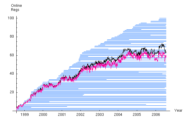
The following graph shows the 8-year history of online REGs in the network. Each blue line represents the period of time a single reg was reporting data. The black trace is the daily sum of online REGs. The red trace is the daily sum of online REGs minus null trials (see also the section on nulls, below). The graph shows the long running history of some nodes as well as the fair number of nodes with short lives. We also can see the actual network growth and how the network changes even with a more or less constant node number. The relatively flat trend beginning in 2004 reflects a decision to maintain the network at about 65-70 nodes, a number that is manageable with available resources.
Random Sources
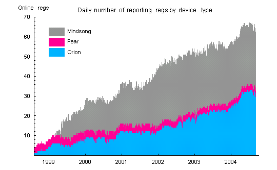
The data are produced by three different makes of electronic random event generators (REG or RNG): Pear, Mindsong and Orion. All data trials are sums of 200 bits. The trialsums are collected once a second at each host site. The Pear and Mindsong devices produce about 12 trials per second and the Orions about 39 (thus 95% of the source data is not collected). REGs are added to the network over time, and the data represent an evolving set of REGs and geographical nodes. The network started with 4 REGs and currently has about 65 in operation. The changing size and distribution of the array contributes to the complexity of some analyses.
Raw Data
The data are available for download from the GCP website using a web-based extract form. Following is a small sample (10 seconds, half the eggs) of the CSV file presented by the form. More detail is available on the data format. Analysts will need further information on file retrieval and processing.
Nulls
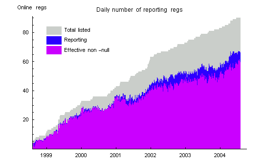
It is fairly common that egg nodes send null trials. Nulls may persist for long times, as when a host site goes down, or may appear intermitently. Nulls do not cause problems for calculations on the data, but they can add to the inherent variability of some statistics.
Database Composition
Some statistics summarizing the dimensions and composition of the database are listed in the following table. (Note: the raw data files list times and values of reg output. This doesn’t constitute a database in the strict sense of the term. We use database in a looser sense, to refer to all the GCP data through Sept. 8, 2004)
| Total Trials | 7.64E+9 |
| Total Nulls | 7.93E+8 |
| Total Non-Null Trials | 6.85E+9 |
| Total Days | 2224.6 |
| Online REG days | 84772 |
| Current REGs Online | 60-65 |
| Average REGs Online/Day | 38.1 |
| Total Events | 183 |
| Total Accepted Events | 170 |
| Z-Score of Accepted Global Events | 4.02 |
Normalizing the Data
The Logical XOR
Ideally, trials distribute like binomial[200, 0.5] (mean 100, variance 50). But although they all are high-quality random sources, this is not necessarily the case for these real-life devices. A logical XOR of the raw bit-stream with a fixed pattern of bits with exactly 0.5 probability compensates mean biases of the REGs. The Pear and Orion REGs use a 01
bitmask and the Mindsong uses a 560-bit mask (the Mindsong mask is the string of all possible 8-bit combinations of 4 0
’s and 4 1
’s. Analysis confirms that the XOR’d data has very good, stable means. XORing does more than correct mean bias. For example, XORing a binomial[N,p] will force the expected p to 0.5, so the variance is transformed as well. That is, if a bias of the mean is compensated by the XOR, this will change the variance proportionally. (See further comments on this point.)
Using the XOR to mitigate possible biases has implications. For example, Jeff Scargle says,
I feel this process rejects the kind of signal that most people probably think is being searched for ... namely consciousness affecting the RNGs ... but because of the XOR, you are only sensitive to consciousness affecting the final data stream. We discussed this before, but I still find it amazing that the entire operation has thrown out at least this baby along with the bathwater.
The two main points I make in response are:
- the XOR is used to exclude an important class of potential spurious effects — biases that might arise from temperature changes, component aging, etc.
- the XOR’d data streams do exhibit anomalous structure in controlled laboratory experiments, as well as in the timeseries we record for the GCP. They do not show extra-chance anomalous structure in calibrations and control sequences.
See also the description of the REG devices used in the GCP, which includes discussion of the XOR procedure’s purposes and implementation. A note responding to skeptical concerns about the XOR contains more technical detail.
Variance Bias
After XOR’ing, the mean is guaranteed over the long run to fit theoretical expectation. The trial variances remain biased, however. The biases are small (about 1 part in 10,000) and generally stable on long timescales. They are corrected by standardization of the trialsums to standard normal variables (z-scores). Mindsong REGs tend to have positive biases. This gives a net positive variance bias to the data. Since the GCP hypothesis explicitly looks for a positive variance bias, there is a requirement for important, albeit small, corrections. The variance biases tell us that the raw, unXOR’d trials cannot be modeled as a simple binomial with shifted bit probability.
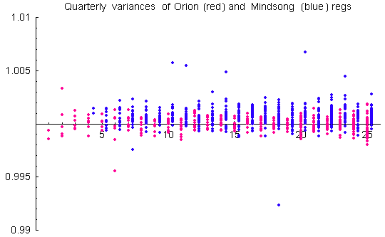
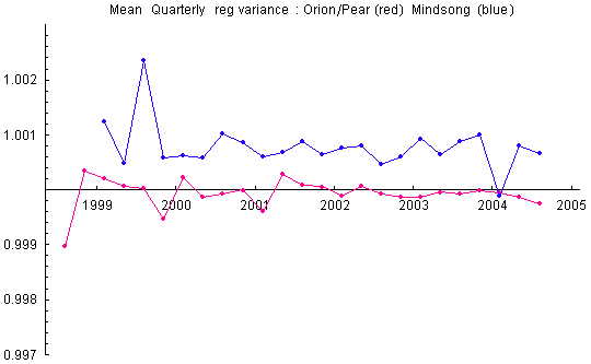
The biases are small, even for the few devices that look like outliers in the figure above, but they are stable, and given large samples of months and years of data, they become statistically significant. We treat them as real biases that need to be corrected by normalization for rigorous analysis. The sensitivity of analyses to variance bias depends on the statistic calculated. Two typical calculations are the trial variance and the variance of the trial means across REGs at 1-second intervals. That is, Var(z) and Var(Z)==Var(Sum(z)), where z are the reg trials and the sum is over all REGs for each second. We sometimes refer to these as the device and network variances, respectively. (Note: when using standardized trial z-scores, there is little difference between variances calculated with respect to theoretical or sample means; theoretical and sample variances will be distinguished where necessary).
Identifying and Addressing Bad Data
Bad Network Days
On a few days, the network produced faulty or incomplete data. These occurred during the first weeks after the GCP began operation and during hacker attack in August 2001. The days August 11, 25, 31 and September 6 have less than 86400 seconds of data. These days are retained in the database. For the days August 5-8, inclusive, the data consists mostly of nulls for all REGs. These days have been removed from the standardized data.
Out-of-bound trials
The REGs occasionally produce improbable trial values. This is usually associated with intermitent hardware problems such as a sudden loss of power during sampling or buffer reads. These trials are removed before analysis. All trialsums that deviate by 45 or more from the theoretical mean of 100 are removed and replaced by nulls.
Rotten Eggs
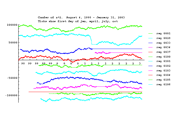
Sections of reg data that do not pass stability criteria are masked and excluded from analysis. Data from these rotten eggs
are usually very obvious, as the next figure shows. There are cases where excluding data is a judgment call. The current criteria impose a limit that will, on average, exclude 0.02% of valid data (an hour or two of data per year). For more detail, contact the Project director, Roger Nelson.
After out-of-bound trials have been removed, the mean and variance of each reg are checked for stability. The links following the image below show graphs of actual data for individual eggs for long periods (up to four years).
Visualizing Effects of Bad Data
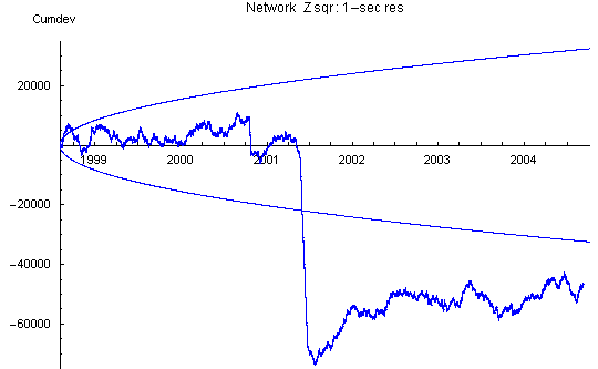
The first two plots below display the effect of bad data from the rotten eggs (with a small contribution from variance bias) on the statistics. Out-of-bounds trials have been removed from the data.
Network Variance
The network Z is the mean trial z-score divided by the square root of the number of trials (i.e., the Stouffer Z). The network Z squared shown here (Network Zsqr) is the variance of the network Z with respect to a theoretical mean of zero. Here the effect of the bad data from rotten eggs is evidenced as steps or spikes in the cumulative deviations.
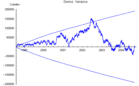
Device Variance
The effect of the reg variance biases is seen most clearly in the device variance plot which has a strong positive slope between bad data steps. The slope increases with time and is roughly proportional to the number of Mindsong REGs in the network, as expected from the tendency to positive bias of these devices.
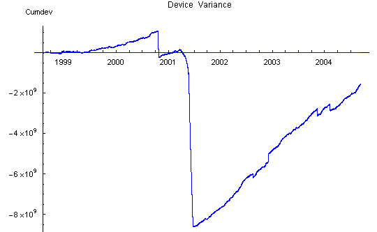
rotten) reg data. The large positive slope is due to variance bias of the individual REGs. This bias is primarily coming from the Mindsong REGs.
Standardized Data
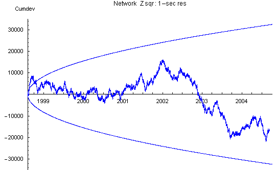
When the rotten eggs and the out-of-bounds trials are removed, and the data are normalized using the empirical variance for each egg, the resulting curves accurately represent the behavior of true random sources. The following figures use the same cumulative deviation presentation as the preceding raw
data, and now we see a random walk that does not exhibit any long term trend. All statistics are well-behaved and lie within 0.05 probability envelopes.
Corrected Network Variance
Here we can see the effect of standardization. The network Z is the mean trial z-score divided by the square root of the number of trials (i.e., the Stouffer Z). The network Z squared shown here (Network Zsqr) is the variance of the network Z with respect to a theoretical mean of zero. Note that the network variance cumulative Z ends off zero because the weighting of REGs is not strictly uniform in the calculation of the Z statistic.
Corrected Device Variance
Again, the standardization removes data defects and leaves clean data fluctuations. The device variance is the sample variance of individual reg trials for 1-sec blocking. The device variance probability envelopes are expanded because the degrees-of-freedom are proportional to the number of REGs online, which grows with time. Note that the device variance cumulative deviation trace ends at zero, as expected for standardized data.
